Statistical comparison of models using grid search#

This example illustrates how to statistically compare the performance of models trained and evaluated using GridSearchCV.

We will start by simulating moon shaped data (where the ideal separation between classes is non-linear), adding to it a moderate degree of noise. Datapoints will belong to one of two possible classes to be predicted by two features. We will simulate 50 samples for each class:

import matplotlib.pyplot as plt
import seaborn as sns

from sklearn.datasets import make_moons

X, y = make_moons(noise=0.352, random_state=1, n_samples=100)

sns.scatterplot(
    x=X[:, 0], y=X[:, 1], hue=y, marker="o", s=25, edgecolor="k", legend=False
).set_title("Data")
plt.show()

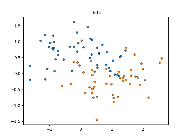
We will compare the performance of SVC estimators that vary on their kernel parameter, to decide which choice of this hyper-parameter predicts our simulated data best. We will evaluate the performance of the models using RepeatedStratifiedKFold, repeating 10 times a 10-fold stratified cross validation using a different randomization of the data in each repetition. The performance will be evaluated using roc_auc_score.

from sklearn.model_selection import GridSearchCV, RepeatedStratifiedKFold
from sklearn.svm import SVC

param_grid = [
    {"kernel": ["linear"]},
    {"kernel": ["poly"], "degree": [2, 3]},
    {"kernel": ["rbf"]},
]

svc = SVC(random_state=0)

cv = RepeatedStratifiedKFold(n_splits=10, n_repeats=10, random_state=0)

search = GridSearchCV(estimator=svc, param_grid=param_grid, scoring="roc_auc", cv=cv)
search.fit(X, y)

GridSearchCV(cv=RepeatedStratifiedKFold(n_repeats=10, n_splits=10, random_state=0),
             estimator=SVC(random_state=0),
             param_grid=[{'kernel': ['linear']},
                         {'degree': [2, 3], 'kernel': ['poly']},
                         {'kernel': ['rbf']}],
             scoring='roc_auc')

In a Jupyter environment, please rerun this cell to show the HTML representation or trust the notebook.
On GitHub, the HTML representation is unable to render, please try loading this page with nbviewer.org.

We can now inspect the results of our search, sorted by their mean_test_score:

import pandas as pd

results_df = pd.DataFrame(search.cv_results_)
results_df = results_df.sort_values(by=["rank_test_score"])
results_df = results_df.set_index(
    results_df["params"].apply(lambda x: "_".join(str(val) for val in x.values()))
).rename_axis("kernel")
results_df[["params", "rank_test_score", "mean_test_score", "std_test_score"]]

	params	rank_test_score	mean_test_score	std_test_score
kernel
rbf	{'kernel': 'rbf'}	1	0.9400	0.079297
linear	{'kernel': 'linear'}	2	0.9300	0.077846
3_poly	{'degree': 3, 'kernel': 'poly'}	3	0.9044	0.098776
2_poly	{'degree': 2, 'kernel': 'poly'}	4	0.6852	0.169106

We can see that the estimator using the 'rbf' kernel performed best, closely followed by 'linear'. Both estimators with a 'poly' kernel performed worse, with the one using a two-degree polynomial achieving a much lower performance than all other models.

Usually, the analysis just ends here, but half the story is missing. The output of GridSearchCV does not provide information on the certainty of the differences between the models. We don’t know if these are statistically significant. To evaluate this, we need to conduct a statistical test. Specifically, to contrast the performance of two models we should statistically compare their AUC scores. There are 100 samples (AUC scores) for each model as we repreated 10 times a 10-fold cross-validation.

However, the scores of the models are not independent: all models are evaluated on the same 100 partitions, increasing the correlation between the performance of the models. Since some partitions of the data can make the distinction of the classes particularly easy or hard to find for all models, the models scores will co-vary.

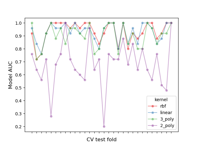
Let’s inspect this partition effect by plotting the performance of all models in each fold, and calculating the correlation between models across folds:

# create df of model scores ordered by performance
model_scores = results_df.filter(regex=r"split\d*_test_score")

# plot 30 examples of dependency between cv fold and AUC scores
fig, ax = plt.subplots()
sns.lineplot(
    data=model_scores.transpose().iloc[:30],
    dashes=False,
    palette="Set1",
    marker="o",
    alpha=0.5,
    ax=ax,
)
ax.set_xlabel("CV test fold", size=12, labelpad=10)
ax.set_ylabel("Model AUC", size=12)
ax.tick_params(bottom=True, labelbottom=False)
plt.show()

# print correlation of AUC scores across folds
print(f"Correlation of models:\n {model_scores.transpose().corr()}")

Correlation of models:
 kernel       rbf    linear    3_poly    2_poly
kernel
rbf     1.000000  0.882561  0.783392  0.351390
linear  0.882561  1.000000  0.746492  0.298688
3_poly  0.783392  0.746492  1.000000  0.355440
2_poly  0.351390  0.298688  0.355440  1.000000

We can observe that the performance of the models highly depends on the fold.

As a consequence, if we assume independence between samples we will be underestimating the variance computed in our statistical tests, increasing the number of false positive errors (i.e. detecting a significant difference between models when such does not exist) [1].

Several variance-corrected statistical tests have been developed for these cases. In this example we will show how to implement one of them (the so called Nadeau and Bengio’s corrected t-test) under two different statistical frameworks: frequentist and Bayesian.

Comparing two models: frequentist approach#

We can start by asking: “Is the first model significantly better than the second model (when ranked by mean_test_score)?”

To answer this question using a frequentist approach we could run a paired t-test and compute the p-value. This is also known as Diebold-Mariano test in the forecast literature [5]. Many variants of such a t-test have been developed to account for the ‘non-independence of samples problem’ described in the previous section. We will use the one proven to obtain the highest replicability scores (which rate how similar the performance of a model is when evaluating it on different random partitions of the same dataset) while maintaining a low rate of false positives and false negatives: the Nadeau and Bengio’s corrected t-test [2] that uses a 10 times repeated 10-fold cross validation [3].

This corrected paired t-test is computed as:

\[t=\frac{\frac{1}{k \cdot r}\sum_{i=1}^{k}\sum_{j=1}^{r}x_{ij}} {\sqrt{(\frac{1}{k \cdot r}+\frac{n_{test}}{n_{train}})\hat{\sigma}^2}}\]

where $k$ is the number of folds, $r$ the number of repetitions in the cross-validation, $x$ is the difference in performance of the models, $n_{test}$ is the number of samples used for testing, $n_{train}$ is the number of samples used for training, and $\hat{\sigma}^2$ represents the variance of the observed differences.

Let’s implement a corrected right-tailed paired t-test to evaluate if the performance of the first model is significantly better than that of the second model. Our null hypothesis is that the second model performs at least as good as the first model.

import numpy as np
from scipy.stats import t


def corrected_std(differences, n_train, n_test):
    """Corrects standard deviation using Nadeau and Bengio's approach.

    Parameters
    ----------
    differences : ndarray of shape (n_samples,)
        Vector containing the differences in the score metrics of two models.
    n_train : int
        Number of samples in the training set.
    n_test : int
        Number of samples in the testing set.

    Returns
    -------
    corrected_std : float
        Variance-corrected standard deviation of the set of differences.
    """
    # kr = k times r, r times repeated k-fold crossvalidation,
    # kr equals the number of times the model was evaluated
    kr = len(differences)
    corrected_var = np.var(differences, ddof=1) * (1 / kr + n_test / n_train)
    corrected_std = np.sqrt(corrected_var)
    return corrected_std


def compute_corrected_ttest(differences, df, n_train, n_test):
    """Computes right-tailed paired t-test with corrected variance.

    Parameters
    ----------
    differences : array-like of shape (n_samples,)
        Vector containing the differences in the score metrics of two models.
    df : int
        Degrees of freedom.
    n_train : int
        Number of samples in the training set.
    n_test : int
        Number of samples in the testing set.

    Returns
    -------
    t_stat : float
        Variance-corrected t-statistic.
    p_val : float
        Variance-corrected p-value.
    """
    mean = np.mean(differences)
    std = corrected_std(differences, n_train, n_test)
    t_stat = mean / std
    p_val = t.sf(np.abs(t_stat), df)  # right-tailed t-test
    return t_stat, p_val

model_1_scores = model_scores.iloc[0].values  # scores of the best model
model_2_scores = model_scores.iloc[1].values  # scores of the second-best model

differences = model_1_scores - model_2_scores

n = differences.shape[0]  # number of test sets
df = n - 1
n_train = len(list(cv.split(X, y))[0][0])
n_test = len(list(cv.split(X, y))[0][1])

t_stat, p_val = compute_corrected_ttest(differences, df, n_train, n_test)
print(f"Corrected t-value: {t_stat:.3f}\nCorrected p-value: {p_val:.3f}")

Corrected t-value: 0.750
Corrected p-value: 0.227

We can compare the corrected t- and p-values with the uncorrected ones:

t_stat_uncorrected = np.mean(differences) / np.sqrt(np.var(differences, ddof=1) / n)
p_val_uncorrected = t.sf(np.abs(t_stat_uncorrected), df)

print(
    f"Uncorrected t-value: {t_stat_uncorrected:.3f}\n"
    f"Uncorrected p-value: {p_val_uncorrected:.3f}"
)

Uncorrected t-value: 2.611
Uncorrected p-value: 0.005

Using the conventional significance alpha level at p=0.05, we observe that the uncorrected t-test concludes that the first model is significantly better than the second.

With the corrected approach, in contrast, we fail to detect this difference.

In the latter case, however, the frequentist approach does not let us conclude that the first and second model have an equivalent performance. If we wanted to make this assertion we need to use a Bayesian approach.

Comparing two models: Bayesian approach#

We can use Bayesian estimation to calculate the probability that the first model is better than the second. Bayesian estimation will output a distribution followed by the mean $\mu$ of the differences in the performance of two models.

To obtain the posterior distribution we need to define a prior that models our beliefs of how the mean is distributed before looking at the data, and multiply it by a likelihood function that computes how likely our observed differences are, given the values that the mean of differences could take.

Bayesian estimation can be carried out in many forms to answer our question, but in this example we will implement the approach suggested by Benavoli and colleagues [4].

One way of defining our posterior using a closed-form expression is to select a prior conjugate to the likelihood function. Benavoli and colleagues [4] show that when comparing the performance of two classifiers we can model the prior as a Normal-Gamma distribution (with both mean and variance unknown) conjugate to a normal likelihood, to thus express the posterior as a normal distribution. Marginalizing out the variance from this normal posterior, we can define the posterior of the mean parameter as a Student’s t-distribution. Specifically:

\[St(\mu;n-1,\overline{x},(\frac{1}{n}+\frac{n_{test}}{n_{train}}) \hat{\sigma}^2)\]

where $n$ is the total number of samples, $\overline{x}$ represents the mean difference in the scores, $n_{test}$ is the number of samples used for testing, $n_{train}$ is the number of samples used for training, and $\hat{\sigma}^2$ represents the variance of the observed differences.

Notice that we are using Nadeau and Bengio’s corrected variance in our Bayesian approach as well.

Let’s compute and plot the posterior:

# initialize random variable
t_post = t(
    df, loc=np.mean(differences), scale=corrected_std(differences, n_train, n_test)
)

Let’s plot the posterior distribution:

x = np.linspace(t_post.ppf(0.001), t_post.ppf(0.999), 100)

plt.plot(x, t_post.pdf(x))
plt.xticks(np.arange(-0.04, 0.06, 0.01))
plt.fill_between(x, t_post.pdf(x), 0, facecolor="blue", alpha=0.2)
plt.ylabel("Probability density")
plt.xlabel(r"Mean difference ($\mu$)")
plt.title("Posterior distribution")
plt.show()

We can calculate the probability that the first model is better than the second by computing the area under the curve of the posterior distribution from zero to infinity. And also the reverse: we can calculate the probability that the second model is better than the first by computing the area under the curve from minus infinity to zero.

better_prob = 1 - t_post.cdf(0)

print(
    f"Probability of {model_scores.index[0]} being more accurate than "
    f"{model_scores.index[1]}: {better_prob:.3f}"
)
print(
    f"Probability of {model_scores.index[1]} being more accurate than "
    f"{model_scores.index[0]}: {1 - better_prob:.3f}"
)

Probability of rbf being more accurate than linear: 0.773
Probability of linear being more accurate than rbf: 0.227

In contrast with the frequentist approach, we can compute the probability that one model is better than the other.

Note that we obtained similar results as those in the frequentist approach. Given our choice of priors, we are essentially performing the same computations, but we are allowed to make different assertions.

Region of Practical Equivalence#

Sometimes we are interested in determining the probabilities that our models have an equivalent performance, where “equivalent” is defined in a practical way. A naive approach [4] would be to define estimators as practically equivalent when they differ by less than 1% in their accuracy. But we could also define this practical equivalence taking into account the problem we are trying to solve. For example, a difference of 5% in accuracy would mean an increase of $1000 in sales, and we consider any quantity above that as relevant for our business.

In this example we are going to define the Region of Practical Equivalence (ROPE) to be $[-0.01, 0.01]$. That is, we will consider two models as practically equivalent if they differ by less than 1% in their performance.

To compute the probabilities of the classifiers being practically equivalent, we calculate the area under the curve of the posterior over the ROPE interval:

rope_interval = [-0.01, 0.01]
rope_prob = t_post.cdf(rope_interval[1]) - t_post.cdf(rope_interval[0])

print(
    f"Probability of {model_scores.index[0]} and {model_scores.index[1]} "
    f"being practically equivalent: {rope_prob:.3f}"
)

Probability of rbf and linear being practically equivalent: 0.432

We can plot how the posterior is distributed over the ROPE interval:

x_rope = np.linspace(rope_interval[0], rope_interval[1], 100)

plt.plot(x, t_post.pdf(x))
plt.xticks(np.arange(-0.04, 0.06, 0.01))
plt.vlines([-0.01, 0.01], ymin=0, ymax=(np.max(t_post.pdf(x)) + 1))
plt.fill_between(x_rope, t_post.pdf(x_rope), 0, facecolor="blue", alpha=0.2)
plt.ylabel("Probability density")
plt.xlabel(r"Mean difference ($\mu$)")
plt.title("Posterior distribution under the ROPE")
plt.show()

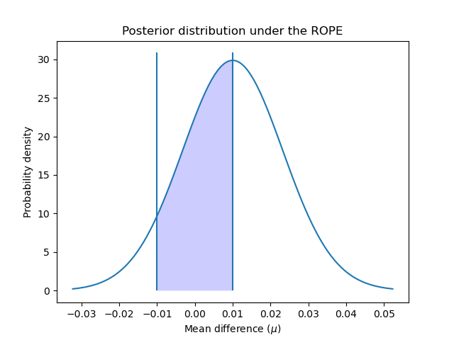
As suggested in [4], we can further interpret these probabilities using the same criteria as the frequentist approach: is the probability of falling inside the ROPE bigger than 95% (alpha value of 5%)? In that case we can conclude that both models are practically equivalent.

The Bayesian estimation approach also allows us to compute how uncertain we are about our estimation of the difference. This can be calculated using credible intervals. For a given probability, they show the range of values that the estimated quantity, in our case the mean difference in performance, can take. For example, a 50% credible interval [x, y] tells us that there is a 50% probability that the true (mean) difference of performance between models is between x and y.

Let’s determine the credible intervals of our data using 50%, 75% and 95%:

cred_intervals = []
intervals = [0.5, 0.75, 0.95]

for interval in intervals:
    cred_interval = list(t_post.interval(interval))
    cred_intervals.append([interval, cred_interval[0], cred_interval[1]])

cred_int_df = pd.DataFrame(
    cred_intervals, columns=["interval", "lower value", "upper value"]
).set_index("interval")
cred_int_df

	lower value	upper value
interval
0.50	0.000977	0.019023
0.75	-0.005422	0.025422
0.95	-0.016445	0.036445

As shown in the table, there is a 50% probability that the true mean difference between models will be between 0.000977 and 0.019023, 70% probability that it will be between -0.005422 and 0.025422, and 95% probability that it will be between -0.016445 and 0.036445.

Pairwise comparison of all models: frequentist approach#

We could also be interested in comparing the performance of all our models evaluated with GridSearchCV. In this case we would be running our statistical test multiple times, which leads us to the multiple comparisons problem.

There are many possible ways to tackle this problem, but a standard approach is to apply a Bonferroni correction. Bonferroni can be computed by multiplying the p-value by the number of comparisons we are testing.

Let’s compare the performance of the models using the corrected t-test:

from itertools import combinations
from math import factorial

n_comparisons = factorial(len(model_scores)) / (
    factorial(2) * factorial(len(model_scores) - 2)
)
pairwise_t_test = []

for model_i, model_k in combinations(range(len(model_scores)), 2):
    model_i_scores = model_scores.iloc[model_i].values
    model_k_scores = model_scores.iloc[model_k].values
    differences = model_i_scores - model_k_scores
    t_stat, p_val = compute_corrected_ttest(differences, df, n_train, n_test)
    p_val *= n_comparisons  # implement Bonferroni correction
    # Bonferroni can output p-values higher than 1
    p_val = 1 if p_val > 1 else p_val
    pairwise_t_test.append(
        [model_scores.index[model_i], model_scores.index[model_k], t_stat, p_val]
    )

pairwise_comp_df = pd.DataFrame(
    pairwise_t_test, columns=["model_1", "model_2", "t_stat", "p_val"]
).round(3)
pairwise_comp_df

	model_1	model_2	t_stat	p_val
0	rbf	linear	0.750	1.000
1	rbf	3_poly	1.657	0.302
2	rbf	2_poly	4.565	0.000
3	linear	3_poly	1.111	0.807
4	linear	2_poly	4.276	0.000
5	3_poly	2_poly	3.851	0.001

We observe that after correcting for multiple comparisons, the only model that significantly differs from the others is '2_poly'. 'rbf', the model ranked first by GridSearchCV, does not significantly differ from 'linear' or '3_poly'.

Pairwise comparison of all models: Bayesian approach#

When using Bayesian estimation to compare multiple models, we don’t need to correct for multiple comparisons (for reasons why see [4]).

We can carry out our pairwise comparisons the same way as in the first section:

pairwise_bayesian = []

for model_i, model_k in combinations(range(len(model_scores)), 2):
    model_i_scores = model_scores.iloc[model_i].values
    model_k_scores = model_scores.iloc[model_k].values
    differences = model_i_scores - model_k_scores
    t_post = t(
        df, loc=np.mean(differences), scale=corrected_std(differences, n_train, n_test)
    )
    worse_prob = t_post.cdf(rope_interval[0])
    better_prob = 1 - t_post.cdf(rope_interval[1])
    rope_prob = t_post.cdf(rope_interval[1]) - t_post.cdf(rope_interval[0])

    pairwise_bayesian.append([worse_prob, better_prob, rope_prob])

pairwise_bayesian_df = pd.DataFrame(
    pairwise_bayesian, columns=["worse_prob", "better_prob", "rope_prob"]
).round(3)

pairwise_comp_df = pairwise_comp_df.join(pairwise_bayesian_df)
pairwise_comp_df

	model_1	model_2	t_stat	p_val	worse_prob	better_prob	rope_prob
0	rbf	linear	0.750	1.000	0.068	0.500	0.432
1	rbf	3_poly	1.657	0.302	0.018	0.882	0.100
2	rbf	2_poly	4.565	0.000	0.000	1.000	0.000
3	linear	3_poly	1.111	0.807	0.063	0.750	0.187
4	linear	2_poly	4.276	0.000	0.000	1.000	0.000
5	3_poly	2_poly	3.851	0.001	0.000	1.000	0.000

Using the Bayesian approach we can compute the probability that a model performs better, worse or practically equivalent to another.

Results show that the model ranked first by GridSearchCV 'rbf', has approximately a 6.8% chance of being worse than 'linear', and a 1.8% chance of being worse than '3_poly'. 'rbf' and 'linear' have a 43% probability of being practically equivalent, while 'rbf' and '3_poly' have a 10% chance of being so.

Similarly to the conclusions obtained using the frequentist approach, all models have a 100% probability of being better than '2_poly', and none have a practically equivalent performance with the latter.

Take-home messages#

Small differences in performance measures might easily turn out to be merely by chance, but not because one model predicts systematically better than the other. As shown in this example, statistics can tell you how likely that is.
When statistically comparing the performance of two models evaluated in GridSearchCV, it is necessary to correct the calculated variance which could be underestimated since the scores of the models are not independent from each other.
A frequentist approach that uses a (variance-corrected) paired t-test can tell us if the performance of one model is better than another with a degree of certainty above chance.
A Bayesian approach can provide the probabilities of one model being better, worse or practically equivalent than another. It can also tell us how confident we are of knowing that the true differences of our models fall under a certain range of values.
If multiple models are statistically compared, a multiple comparisons correction is needed when using the frequentist approach.

References