FeatureHasher and DictVectorizer Comparison#

In this example we illustrate text vectorization, which is the process of representing non-numerical input data (such as dictionaries or text documents) as vectors of real numbers.

We first compare FeatureHasher and DictVectorizer by using both methods to vectorize text documents that are preprocessed (tokenized) with the help of a custom Python function.

Later we introduce and analyze the text-specific vectorizers HashingVectorizer, CountVectorizer and TfidfVectorizer that handle both the tokenization and the assembling of the feature matrix within a single class.

The objective of the example is to demonstrate the usage of text vectorization API and to compare their processing time. See the example scripts Classification of text documents using sparse features and Clustering text documents using k-means for actual learning on text documents.

# Author: Lars Buitinck
#         Olivier Grisel <olivier.grisel@ensta.org>
#         Arturo Amor <david-arturo.amor-quiroz@inria.fr>
# License: BSD 3 clause

Load Data#

We load data from The 20 newsgroups text dataset, which comprises around 18000 newsgroups posts on 20 topics split in two subsets: one for training and one for testing. For the sake of simplicity and reducing the computational cost, we select a subset of 7 topics and use the training set only.

from sklearn.datasets import fetch_20newsgroups

categories = [
    "alt.atheism",
    "comp.graphics",
    "comp.sys.ibm.pc.hardware",
    "misc.forsale",
    "rec.autos",
    "sci.space",
    "talk.religion.misc",
]

print("Loading 20 newsgroups training data")
raw_data, _ = fetch_20newsgroups(subset="train", categories=categories, return_X_y=True)
data_size_mb = sum(len(s.encode("utf-8")) for s in raw_data) / 1e6
print(f"{len(raw_data)} documents - {data_size_mb:.3f}MB")

Loading 20 newsgroups training data
3803 documents - 6.245MB

Define preprocessing functions#

A token may be a word, part of a word or anything comprised between spaces or symbols in a string. Here we define a function that extracts the tokens using a simple regular expression (regex) that matches Unicode word characters. This includes most characters that can be part of a word in any language, as well as numbers and the underscore:

import re


def tokenize(doc):
    """Extract tokens from doc.

    This uses a simple regex that matches word characters to break strings
    into tokens. For a more principled approach, see CountVectorizer or
    TfidfVectorizer.
    """
    return (tok.lower() for tok in re.findall(r"\w+", doc))


list(tokenize("This is a simple example, isn't it?"))

['this', 'is', 'a', 'simple', 'example', 'isn', 't', 'it']

We define an additional function that counts the (frequency of) occurrence of each token in a given document. It returns a frequency dictionary to be used by the vectorizers.

from collections import defaultdict


def token_freqs(doc):
    """Extract a dict mapping tokens from doc to their occurrences."""

    freq = defaultdict(int)
    for tok in tokenize(doc):
        freq[tok] += 1
    return freq


token_freqs("That is one example, but this is another one")

defaultdict(<class 'int'>, {'that': 1, 'is': 2, 'one': 2, 'example': 1, 'but': 1, 'this': 1, 'another': 1})

Observe in particular that the repeated token "is" is counted twice for instance.

Breaking a text document into word tokens, potentially losing the order information between the words in a sentence is often called a Bag of Words representation.

DictVectorizer#

First we benchmark the DictVectorizer, then we compare it to FeatureHasher as both of them receive dictionaries as input.

from time import time

from sklearn.feature_extraction import DictVectorizer

dict_count_vectorizers = defaultdict(list)

t0 = time()
vectorizer = DictVectorizer()
vectorizer.fit_transform(token_freqs(d) for d in raw_data)
duration = time() - t0
dict_count_vectorizers["vectorizer"].append(
    vectorizer.__class__.__name__ + "\non freq dicts"
)
dict_count_vectorizers["speed"].append(data_size_mb / duration)
print(f"done in {duration:.3f} s at {data_size_mb / duration:.1f} MB/s")
print(f"Found {len(vectorizer.get_feature_names_out())} unique terms")

done in 1.041 s at 6.0 MB/s
Found 47928 unique terms

The actual mapping from text token to column index is explicitly stored in the .vocabulary_ attribute which is a potentially very large Python dictionary:

type(vectorizer.vocabulary_)

len(vectorizer.vocabulary_)

vectorizer.vocabulary_["example"]

FeatureHasher#

Dictionaries take up a large amount of storage space and grow in size as the training set grows. Instead of growing the vectors along with a dictionary, feature hashing builds a vector of pre-defined length by applying a hash function h to the features (e.g., tokens), then using the hash values directly as feature indices and updating the resulting vector at those indices. When the feature space is not large enough, hashing functions tend to map distinct values to the same hash code (hash collisions). As a result, it is impossible to determine what object generated any particular hash code.

Because of the above it is impossible to recover the original tokens from the feature matrix and the best approach to estimate the number of unique terms in the original dictionary is to count the number of active columns in the encoded feature matrix. For such a purpose we define the following function:

import numpy as np


def n_nonzero_columns(X):
    """Number of columns with at least one non-zero value in a CSR matrix.

    This is useful to count the number of features columns that are effectively
    active when using the FeatureHasher.
    """
    return len(np.unique(X.nonzero()[1]))

The default number of features for the FeatureHasher is 2**20. Here we set n_features = 2**18 to illustrate hash collisions.

FeatureHasher on frequency dictionaries

from sklearn.feature_extraction import FeatureHasher

t0 = time()
hasher = FeatureHasher(n_features=2**18)
X = hasher.transform(token_freqs(d) for d in raw_data)
duration = time() - t0
dict_count_vectorizers["vectorizer"].append(
    hasher.__class__.__name__ + "\non freq dicts"
)
dict_count_vectorizers["speed"].append(data_size_mb / duration)
print(f"done in {duration:.3f} s at {data_size_mb / duration:.1f} MB/s")
print(f"Found {n_nonzero_columns(X)} unique tokens")

done in 0.566 s at 11.0 MB/s
Found 43873 unique tokens

The number of unique tokens when using the FeatureHasher is lower than those obtained using the DictVectorizer. This is due to hash collisions.

The number of collisions can be reduced by increasing the feature space. Notice that the speed of the vectorizer does not change significantly when setting a large number of features, though it causes larger coefficient dimensions and then requires more memory usage to store them, even if a majority of them is inactive.

t0 = time()
hasher = FeatureHasher(n_features=2**22)
X = hasher.transform(token_freqs(d) for d in raw_data)
duration = time() - t0

print(f"done in {duration:.3f} s at {data_size_mb / duration:.1f} MB/s")
print(f"Found {n_nonzero_columns(X)} unique tokens")

done in 0.569 s at 11.0 MB/s
Found 47668 unique tokens

We confirm that the number of unique tokens gets closer to the number of unique terms found by the DictVectorizer.

FeatureHasher on raw tokens

Alternatively, one can set input_type="string" in the FeatureHasher to vectorize the strings output directly from the customized tokenize function. This is equivalent to passing a dictionary with an implied frequency of 1 for each feature name.

t0 = time()
hasher = FeatureHasher(n_features=2**18, input_type="string")
X = hasher.transform(tokenize(d) for d in raw_data)
duration = time() - t0
dict_count_vectorizers["vectorizer"].append(
    hasher.__class__.__name__ + "\non raw tokens"
)
dict_count_vectorizers["speed"].append(data_size_mb / duration)
print(f"done in {duration:.3f} s at {data_size_mb / duration:.1f} MB/s")
print(f"Found {n_nonzero_columns(X)} unique tokens")

done in 0.535 s at 11.7 MB/s
Found 43873 unique tokens

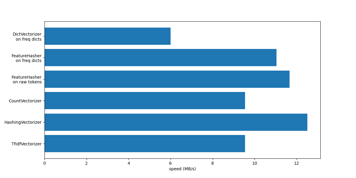
We now plot the speed of the above methods for vectorizing.

import matplotlib.pyplot as plt

fig, ax = plt.subplots(figsize=(12, 6))

y_pos = np.arange(len(dict_count_vectorizers["vectorizer"]))
ax.barh(y_pos, dict_count_vectorizers["speed"], align="center")
ax.set_yticks(y_pos)
ax.set_yticklabels(dict_count_vectorizers["vectorizer"])
ax.invert_yaxis()
_ = ax.set_xlabel("speed (MB/s)")

In both cases FeatureHasher is approximately twice as fast as DictVectorizer. This is handy when dealing with large amounts of data, with the downside of losing the invertibility of the transformation, which in turn makes the interpretation of a model a more complex task.

The FeatureHeasher with input_type="string" is slightly faster than the variant that works on frequency dict because it does not count repeated tokens: each token is implicitly counted once, even if it was repeated. Depending on the downstream machine learning task, it can be a limitation or not.

Comparison with special purpose text vectorizers#

CountVectorizer accepts raw data as it internally implements tokenization and occurrence counting. It is similar to the DictVectorizer when used along with the customized function token_freqs as done in the previous section. The difference being that CountVectorizer is more flexible. In particular it accepts various regex patterns through the token_pattern parameter.

from sklearn.feature_extraction.text import CountVectorizer

t0 = time()
vectorizer = CountVectorizer()
vectorizer.fit_transform(raw_data)
duration = time() - t0
dict_count_vectorizers["vectorizer"].append(vectorizer.__class__.__name__)
dict_count_vectorizers["speed"].append(data_size_mb / duration)
print(f"done in {duration:.3f} s at {data_size_mb / duration:.1f} MB/s")
print(f"Found {len(vectorizer.get_feature_names_out())} unique terms")

done in 0.654 s at 9.5 MB/s
Found 47885 unique terms

We see that using the CountVectorizer implementation is approximately twice as fast as using the DictVectorizer along with the simple function we defined for mapping the tokens. The reason is that CountVectorizer is optimized by reusing a compiled regular expression for the full training set instead of creating one per document as done in our naive tokenize function.

Now we make a similar experiment with the HashingVectorizer, which is equivalent to combining the “hashing trick” implemented by the FeatureHasher class and the text preprocessing and tokenization of the CountVectorizer.

from sklearn.feature_extraction.text import HashingVectorizer

t0 = time()
vectorizer = HashingVectorizer(n_features=2**18)
vectorizer.fit_transform(raw_data)
duration = time() - t0
dict_count_vectorizers["vectorizer"].append(vectorizer.__class__.__name__)
dict_count_vectorizers["speed"].append(data_size_mb / duration)
print(f"done in {duration:.3f} s at {data_size_mb / duration:.1f} MB/s")

done in 0.499 s at 12.5 MB/s

We can observe that this is the fastest text tokenization strategy so far, assuming that the downstream machine learning task can tolerate a few collisions.

TfidfVectorizer#

In a large text corpus, some words appear with higher frequency (e.g. “the”, “a”, “is” in English) and do not carry meaningful information about the actual contents of a document. If we were to feed the word count data directly to a classifier, those very common terms would shadow the frequencies of rarer yet more informative terms. In order to re-weight the count features into floating point values suitable for usage by a classifier it is very common to use the tf-idf transform as implemented by the TfidfTransformer. TF stands for “term-frequency” while “tf-idf” means term-frequency times inverse document-frequency.

We now benchmark the TfidfVectorizer, which is equivalent to combining the tokenization and occurrence counting of the CountVectorizer along with the normalizing and weighting from a TfidfTransformer.

from sklearn.feature_extraction.text import TfidfVectorizer

t0 = time()
vectorizer = TfidfVectorizer()
vectorizer.fit_transform(raw_data)
duration = time() - t0
dict_count_vectorizers["vectorizer"].append(vectorizer.__class__.__name__)
dict_count_vectorizers["speed"].append(data_size_mb / duration)
print(f"done in {duration:.3f} s at {data_size_mb / duration:.1f} MB/s")
print(f"Found {len(vectorizer.get_feature_names_out())} unique terms")

done in 0.654 s at 9.5 MB/s
Found 47885 unique terms

Summary#

Let’s conclude this notebook by summarizing all the recorded processing speeds in a single plot:

fig, ax = plt.subplots(figsize=(12, 6))

y_pos = np.arange(len(dict_count_vectorizers["vectorizer"]))
ax.barh(y_pos, dict_count_vectorizers["speed"], align="center")
ax.set_yticks(y_pos)
ax.set_yticklabels(dict_count_vectorizers["vectorizer"])
ax.invert_yaxis()
_ = ax.set_xlabel("speed (MB/s)")

Notice from the plot that TfidfVectorizer is slightly slower than CountVectorizer because of the extra operation induced by the TfidfTransformer.

Also notice that, by setting the number of features n_features = 2**18, the HashingVectorizer performs better than the CountVectorizer at the expense of inversibility of the transformation due to hash collisions.

We highlight that CountVectorizer and HashingVectorizer perform better than their equivalent DictVectorizer and FeatureHasher on manually tokenized documents since the internal tokenization step of the former vectorizers compiles a regular expression once and then reuses it for all the documents.

Total running time of the script: (0 minutes 4.981 seconds)

Related examples